Self-Supervised Monocular Depth Estimation

In October of 2020, I learned of strategy to use monocular depth estimation as a cheaper low-accuracy alternative to LIDAR. Essentially, you can use a camera and a self-supervised monocular depth estimation network to produce colour images with depth information (RGBD images). Since we know camera’s exact position and orientation, each pixel in the RGBD image can be projected into 3d to form a pseudo-pointcloud with RGB+XY information. This is similar to how the Xbox Kinect obtains 3d information, though the Kinect uses infrared sensors to gauge depth instead of a RGBD image. With this pseudo-pointcloud, we can use Simultaneous Localization and Mapping (SLAM) or Occupancy Grid algorithms to produce a 3d map of our environment with colour information.

Above: RGBD mapping with the XBOX Kinect

At the same time, I was taking CS484 (Computational Vision) taught by Professor Yuri Boykov. CS484 provides a very in-depth look into classical computer vision and focuses on camera geometry (pinhole camera model, projections and transformations, and epipolar geometry). Conveniently, just a couple weeks after I heard of the concept, we learned the core concepts behind self-supervised monocular depth estimation. The main paper we focused on was Godard et al.’s 2017 paper titled Unsupervised Monocular Depth Estimation with Left-Right Consistency. For my CS484 final project, I wanted to minimally reproduce the results in the paper while clearly explaining in a step-by-step manner exactly how the model functions. You can find my project on my github.

Dense Stereo Reconstruction

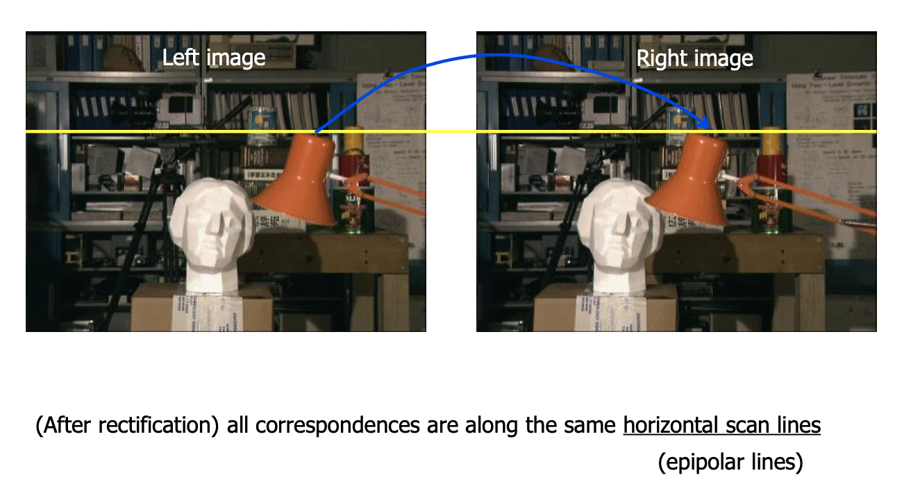
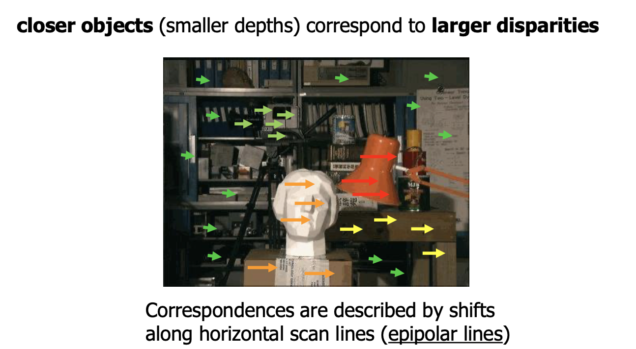
First, some context. It’s pretty easy to compute depth information without a neural network given two camera images where the cameras have known position. This is called Stereo Reconstruction. Assuming either the cameras are perfectly parallel or the images have been rectified, points along a horizontal scan-line in the left image will correspond to points along the horizontal scan-line in the right image. Since we have two cameras at varying positions, near objects will have a larger disparity between the left and right images than far objects. The depth of a certain pixel in question is then directly proportional to this disparity value. If your cameras are parallel (no rectification) and F = focal length (m), B = baseline distance (m), d = disparity (pixels), then depth = (b * f) / d (source).

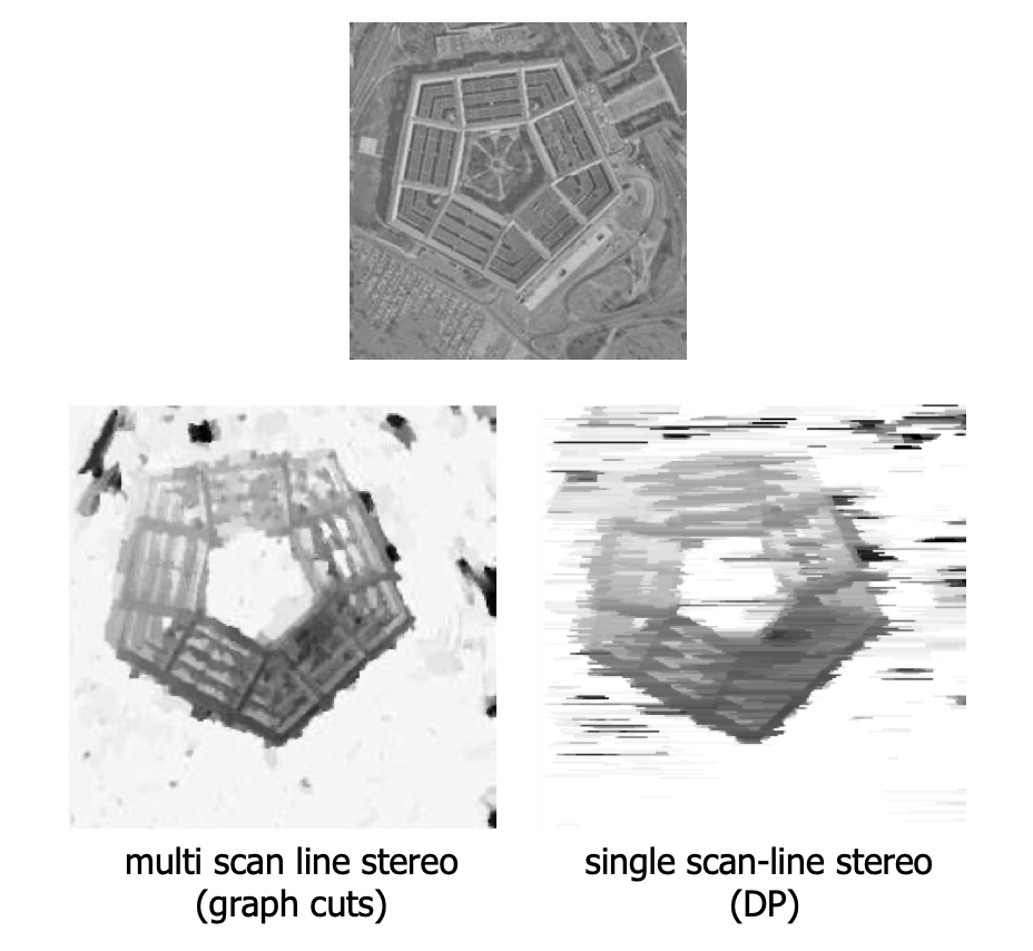
But, there are some issues with this approach. First of all, some pixels are visible in one image but occluded in the other. This is a loss of information. Secondly, disparity values are calculated on a scanline-by-scanline basis, so there is no guarantee that scanlines next to each other will have consistent depths. This leads to “Streaking” artifacts in the final disparity map. Thirdly, it’s really hard to tell the disparity level of areas with uniform texture. Some of these issues (such as the streaking) can be resolved by enforcing multi-scanline consistency using regularization and graph-cuts.

Self-supervised monocular depth estimation

Machine learning can do Much better. By leveraging past experiences, humans can extract pretty good depth information using only one eye or a single image. Deep learning can do the same thing. However, humans have years and years of experience to learn these depth queues. in contrast, it’s very difficult to get datasets with depth information large enough to train a supervised depth estimation network. Each pixel in each image needs to be classified with the correct disparity, which is really expensive. To solve this issue, we remove the requirement for accurate ground truth, and instead create a self-supervised network.

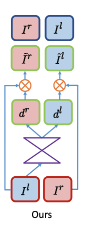
Godard et al.’s primary contribution is a novel loss-function for self-supervised monocular depth estimation that enforces left-right photo consistency. During training, we use left-right image pair taken by a set of parallel cameras with a known base-length. The KITTI Dataset has over 29,000 such left-right image pairs. The goal of the network is to use one of the images (in this case, the left image) to estimate two disparity maps. One disparity map contains the disparity values from the left image to the right image, and the other contains the disparity values from the right image to the left image. Note that the left-to-right disparity map allows us to reconstruct the right image using the left image by applying the appropriate disparity values. Similarly, the right-to-left disparity map allows us to reconstruct the left image using the right image. These “reconstructed images” can be compared with the original images to evaluate the accuracy of the disparity map. This comparison is the main component of the loss function. Using both the reconstructed left and right images allows the network to enforce consistency between it’s predictions. This reduces artifacts in the disparity maps that would occur if we only used one reconstructed image (instead of two).

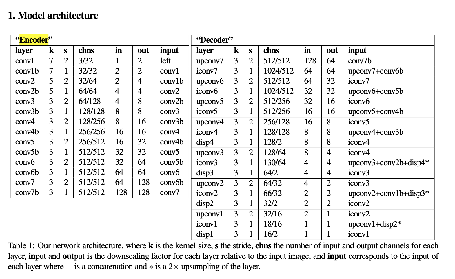
The model itself is actually pretty straight forwards, a basic convolutional encoder-decoder architecture using the ResNet encoder and a lot of skip connections for resolution.

For brevity, I’ve left out a bunch of the other details and improvements that Godard et al. made. See my project on github a more complete demo and explanation or read the paper here.

Results

After training for 10 epochs on a small subset of the KITTI dataset (5268 left/right image pairs), I achieved the following results. Note that yellow = high disparity, blue = low disparity. These are some pretty good results for such little training! You can clearly see that the disparities are roughly correct and the vanishing point of the street is accurately represented. However, the output disparity map is pretty fuzzy, and the left disparity map has sharp lines on edge boundaries while the right disparity map does not. Some of the disparities are also wrong or inverted (for example, model predicts that the white banners on the right are inset into the wall instead of protruding).

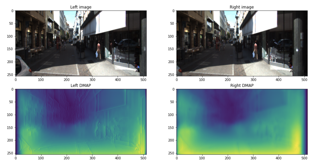
These issues would likely be solved by more training time on a larger dataset. Training for 50 epochs over the entire KITTI dataset (~29,000 left-right pairs), the authors were able to achieve amazing results.

CS484 and this project sparked my interest in the creative ways that computer vision can be applied for autonomous driving. There’s a lot of mathematics and geometry behind the classic computer vision approaches, and I’m starting to believe that a combined approach using both classic geometric computer vision with new deep neural networks is the way forward.

Readings:

1. Unsupervised Monocular Depth Estimation with Left-Right Consistency: https://arxiv.org/pdf/1609.03677v3.pdf
2. Open3d RGBD Images: http://www.open3d.org/docs/latest/tutorial/Basic/rgbd_image.html
3. KITTI Dataset: http://www.cvlibs.net/datasets/kitti/index.php
4. MonoDepth repository: https://github.com/mrharicot/monodepth
5. CS484 Course Notes for Dense Stereo Reconstruction: https://cs.uwaterloo.ca/~yboykov/Courses/cs484_2018/Lectures/lec08_stereo_u.pdf